Note:
This page was generated from a Jupyter notebook which can be found at
docs/tutorial_notebooks/4_BayesLOSVD.ipynb
in your DYNAMITE directory.
—-
4. BayesLOSVD and DYNAMITE
This notebook will show how to run DYNAMITE orbit-based models using BayesLOSVD output. BayesLOSVD is a Python library for the non-parametric extraction of the Line-Of-Sight Velocity Distributions (LOSVDs) in galaxies. Rather than describe the LOSVD using Gauss-Hermite expansion, BayesLOSVD represents the LOSVD in a histogram format.
An example galaxy: NGC4550
We will model the galaxy NGC4550, which has a complex LOSVD. The following is taken from Figure 7 of Falcón-Barroso & Martig 2020, showing LOSVDs extracted using BayesLOSVD at three regions,
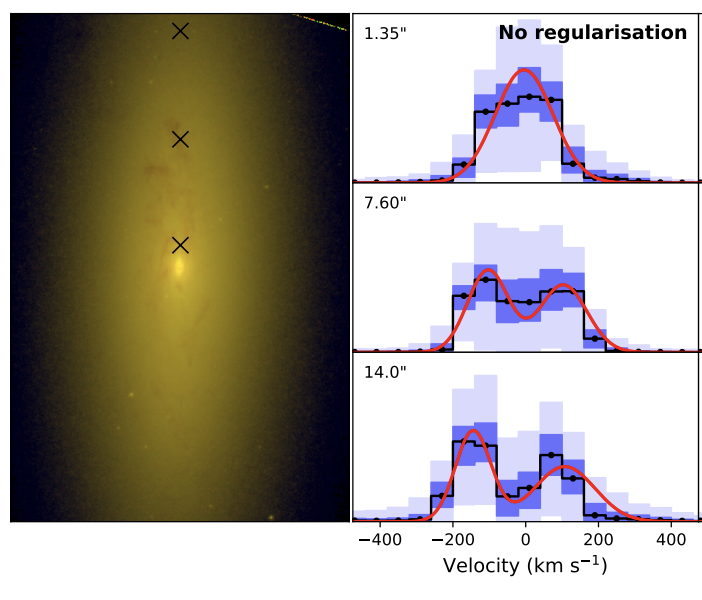
We see clearly bimodal LOSVDs in the galaxy outskirts, indicating a strong counter-rotating stellar component.
Data preparation
We require the *_results.hdf5 output file from BayesLOSVD. Two such files for NGC4550 have been kindly provided by Jesus Falcón-Barroso, and can be found in the directory NGC4550_input. They differ in the form of LOSVD regularisation used, - NGC4550_SAURON-SP_results.hdf5: using simplex regularisation - NGC4550_SAURON-RW_results.hdf5: using random walk regularisation
These *_results.hdf5 files contains LOSVD constraints for all spatial regions. For more details, and instructions on creating your own *_results.hdf5 files, see the BayesLOSVD documentation.
To prepare this data for use in DYNAMITE, we must
convert kinematics to Astropy ECSV file format
add the PSF to the kinematics file header
create the auxillary
aperture.datandbins.datfilesget MGE data (in Astropy ECSV format)
This can be done as follows,
[1]:
import numpy as np
import matplotlib.pyplot as plt
from scipy import stats
import dynamite as dyn
print('Using DYNAMITE version:', dyn.__version__)

BayesLOSVD = dyn.kinematics.BayesLOSVD(hist_width=1,
                                       hist_center=0,
                                       hist_bins=0,
                                       type='BayesLOSVD')
infile = 'NGC4550_input/NGC4550_SAURON-SP_results.hdf5'
outfile = 'NGC4550_input/dynamite_input/bayes_losvd_kins.ecsv'
BayesLOSVD.write_losvds_to_ecsv_format(infile, outfile=outfile)
Using DYNAMITE version: 4.3.0
We next add the PSF to the kinematics. The seeing - from Table 3 of Emsellem et al 2004 - has FWHM of 2.1 arcsec. We convert this to a Gaussian sigma, and add to the header of the kinematics file,
[2]:
seeing_fwhm = 2.1
seeing_gauss_sigma = seeing_fwhm/2.35
# add the psf to file header
BayesLOSVD.add_psf_to_datafile(sigma=[seeing_gauss_sigma],
                               weight=[1.],
                               datafile=outfile)

# re-create the BayesLOSVD object reading in the complete kinematics file
BayesLOSVD = dyn.kinematics.BayesLOSVD(datafile=outfile,
                                       type='BayesLOSVD')
Next create the auxillary aperture.dat and bins.dat files. This will require the galaxy’s position angle. Table 3 of Emsellem et al 2004, gives PA = 0.
[3]:
position_angle = 0.
angle_deg = 90. - position_angle
dyn_input_direc = 'NGC4550_input/dynamite_input/'
BayesLOSVD.write_aperture_and_bin_files(filename=infile,
                                        angle_deg=angle_deg,
                                        aperture_filename=dyn_input_direc+'aperture.dat',
                                        bin_filename=dyn_input_direc+'bins.dat')
Finally we need the Multi Gaussian Expansion. MGEs for Atlas3D galaxies (including NGC4550) can be found under the link for the MGE parameters for the deconvolved r-band surface brightness on the Atlas3D page. The MGE NGC4550 is provided in NGC4550_input/dynamite_input/. We have already manually copied and pasted the MGE-data into the required Astropy ECSV format.
The input directory NGC4550_input/dynamite_input/ now contains all 4 required files: - mge.ecsv - bayes_losvd_kins.ecsv - aperture.dat - bins.dat
A look at the BayesLOSVD data
We can take a look at the BayesLOSVD data. The data can be found in the file NGC4550_input/dynamite_input/bayes_losvd_kins.ecsv, which we defined as outfile above. First let’s read the data-files and auxiliary files, into a dyn.kinematics.BayesLOSVD objects,
[4]:
BayesLOSVD = dyn.kinematics.BayesLOSVD(datafile=outfile,
                                       aperturefile=dyn_input_direc+'aperture.dat',
                                       binfile=dyn_input_direc+'bins.dat',
                                       type='BayesLOSVD')
The table has one row per spatial (in this case Voronoi) bin, and the following columns:
binID_BayesLOSVD: the bin ID used internally in BayesLOSVD
binID_dynamite: the bin ID used internally in DYNAMITE
v: the mean velocity in the bin
sigma: the velocity dispersion in the bin
xbin/ybin : the co-ords of the bin centers
losvd: array holding the LOSVD
dlosvd: array holding LOSVD uncertainties, given by 68% credible intervals per velocity bin (assumed independent)
BayesLOSVD represents the LOSVD as a sequence of weights. Details of the velocity array are stored as metadata to the data table. Details of the LOSVD velocity array are stored as metadata to the data table,
[5]:
print('Bayes-LOSVD table contains meta-data about: ', BayesLOSVD.data.meta.keys())
print('     velocity spacing of bins = ', BayesLOSVD.data.meta['dv'])
print('     number of spatial bins = ', BayesLOSVD.data.meta['nbins'])
print('     number of velocty bins = ', BayesLOSVD.data.meta['nvbins'])
print('     velocity dispersion in the bins = ', BayesLOSVD.data.meta['PSF']['sigma'])
print('     etc...')
Bayes-LOSVD table contains meta-data about:  odict_keys(['dv', 'nbins', 'nvbins', 'vcent', 'PSF'])
     velocity spacing of bins =  60.0
     number of spatial bins =  196
     number of velocty bins =  23
     velocity dispersion in the bins =  [0.8936170212765957]
     etc...
To plot kinematic maps, we can get get the map_plotter function from the kinematics object,
[6]:
map_plotter = BayesLOSVD.get_map_plotter()
map_plotter(BayesLOSVD.data['v'],
            cmap='sauron',
            vmin=-100,
            vmax=100,
            colorbar=True)
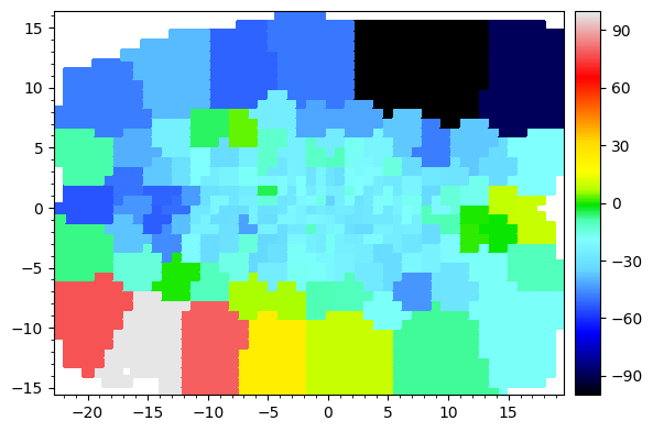
The velocity map is not centered at 0. Let’s center at the galaxy’s systemic velocity. We could either provide this directly, or specify that we want the flux_weighted mean velocity calculated from the kinematic data itself,
[7]:
BayesLOSVD.center_v_systemic(v_systemic='flux_weighted')
BayesLOSVD.save_data_table(outfile)
[8]:
map_plotter(BayesLOSVD.data['v'],
            cmap='sauron',
            vmin=-70,
            vmax=70,
            colorbar=True)
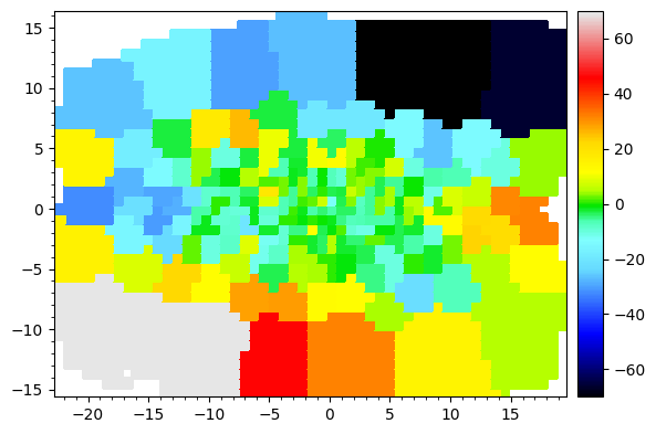
And we can pick a specific bin, and plot the LOSVD there,
[9]:
bin_id = 105

losvd_i = BayesLOSVD.data['losvd'][bin_id,:]
dlosvd_i = BayesLOSVD.data['dlosvd'][bin_id,:]
vcent = BayesLOSVD.data.meta['vcent']
plt.plot(vcent, losvd_i, '-k', label='median')
plt.plot(vcent, losvd_i+dlosvd_i, ':k', label='68% cred. ints.')
plt.plot(vcent, losvd_i-dlosvd_i, ':k')
plt.gca().set_xlabel('Velocity [km/s]')
plt.gca().set_ylabel('LOSVD [km/s]')
_ = plt.gca().set_title(f'LOSVD with 68% CIs in bin {bin_id}')
plt.gca().legend()
plt.show()
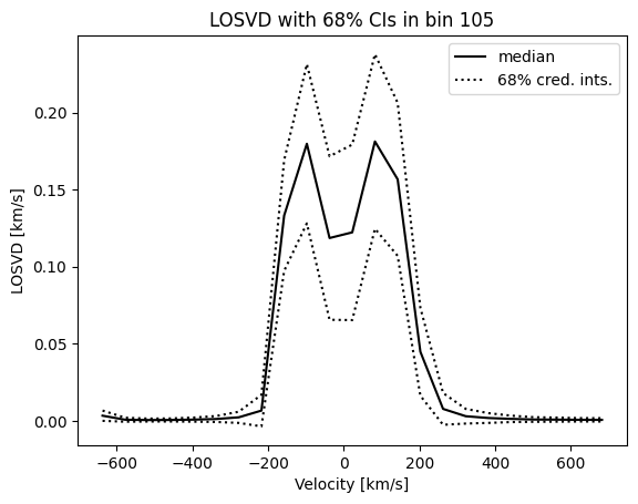
For bin_id=105 we see that the galaxy has a bimodal LOSVD (albeit with quite large uncertainties).
The following are technical notes about BayesLOSVD data. If you’re mainly interested in running DYNAMITE, you can skip below to the section Running DYNAMITE.
Note 1: bin ID’s
The differences between binID_BayesLOSVD and binID_DYNAMITE are that: - binID_BayesLOSVD are zero-indexed, binID_DYNAMITE one-indexed. This is for compatibility with Fortran code, - binID_BayesLOSVD may have some gaps (as some bins may be masked) while DYNAMITE assumes the binIDs increase without gaps. You shouldn’t need to worry about this difference as bin IDs are handled internally, but be aware of the difference for any later analysis.
Note 2: LOSVD normalisations
BayesLOSVD samples the multi-dimensional posterior on the LOSVD weights \(L_i\). The full multidimensional posterior is not saved by defaut, however. What is saved, and what is given in the table above, is the median and 68% Bayesian credible intervals for the weight in each velocity bin.
One important effect of this is on LOSVD normalisation. The posterior samples created by BayesLOSVD are normnalised to 1 i.e.
(this is acheieved by using the simplex datatype in STAN). The default results file, however, gives median values per velocity bin. These are not normalised the same way. Let’s call these median value,
and look at a histogram of the sums of the \(l_i\) in each spatial bin,
[10]:
plt.hist(np.sum(BayesLOSVD.data['losvd'], 1))
plt.axvline(1., ls='--', color='r')
plt.gca().set_xlabel(r'$\sum_i l_{i}$')
plt.gca().set_ylabel('$N$')
plt.gca().set_xlim(0, 1.1)
_ = plt.gca().set_title('LOSVD normalisation in different spatial bins')
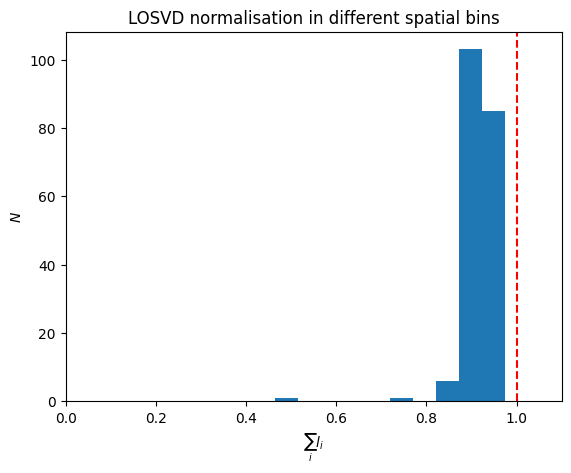
This peaks around 0.9 and, in some cases, is as low as 0.5.
Note 3: calculating moments
When calculating LOSVD moments, we must acccount for the fact that LOSVDs are not normalised. Let’s define the normalised LOSVD as
The quantity \(\hat{l}_{i}\) is what we have used to make point estimates of the the LOSVD mean and standard deviation, which appear in the v and sigma columns of the data-table,
Note 4: inflated velocity dispersions
Let’s compare the BayesLOSVD result with a Gaussian LOSVD approximation in a particular bin,
[11]:
bin_id = 100

# plot BayesLOSVD result
losvd_i = BayesLOSVD.data['losvd'][bin_id,:]
dlosvd_i = BayesLOSVD.data['dlosvd'][bin_id,:]
vcent = BayesLOSVD.data.meta['vcent']
plt.plot(vcent, losvd_i, '-k', label='median')
plt.plot(vcent, losvd_i+dlosvd_i, ':k', label='68% cred. ints.')
plt.plot(vcent, losvd_i-dlosvd_i, ':k')

# plot Gaussian approximation
v = BayesLOSVD.data['v'][bin_id]
sigma = BayesLOSVD.data['sigma'][bin_id]
nrm = stats.norm(v, sigma)
pdf = nrm.pdf(vcent)
plt.gca().plot(vcent, pdf/np.sum(pdf), color='r', ls='--', label='Gauss. approx.')

# labels
plt.gca().set_xlabel('Velocity [km/s]')
plt.gca().set_ylabel('LOSVD [km/s]')
_ = plt.gca().set_title(f'LOSVD with 68% CIs in bin {bin_id}')
plt.gca().legend()
plt.show()
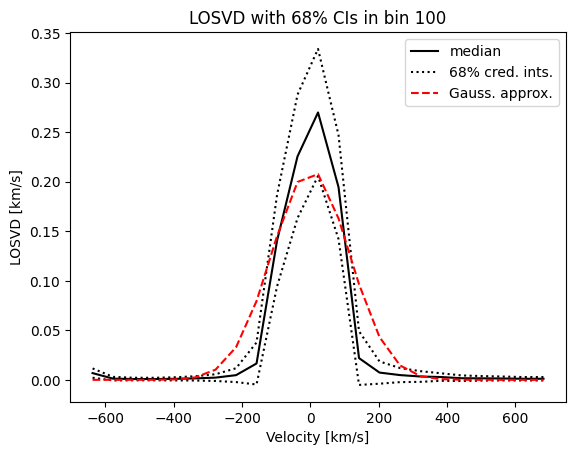
The Gaussian approximation is much wider then the median BayesLOSVD result. Why is this? Let’s look at the this plot again, this time on a log-scale,
[12]:
bin_id = 100

# plot BayesLOSVD result
losvd_i = BayesLOSVD.data['losvd'][bin_id,:]
dlosvd_i = BayesLOSVD.data['dlosvd'][bin_id,:]
vcent = BayesLOSVD.data.meta['vcent']
plt.plot(vcent, losvd_i, '-k', label='median')
plt.plot(vcent, losvd_i+dlosvd_i, ':k', label='68% cred. ints.')
plt.plot(vcent, losvd_i-dlosvd_i, ':k')

# plot Gaussian approximation
v = BayesLOSVD.data['v'][bin_id]
sigma = BayesLOSVD.data['sigma'][bin_id]
nrm = stats.norm(v, sigma)
pdf = nrm.pdf(vcent)
plt.gca().plot(vcent, pdf/np.sum(pdf), color='r', ls='--', label='Gauss. approx.')

# labels
plt.gca().set_xlabel('Velocity [km/s]')
plt.gca().set_ylabel('LOSVD [km/s]')
_ = plt.gca().set_title(f'LOSVD with 68% CIs in bin {bin_id}')
plt.gca().legend()
plt.gca().set_yscale('log')
plt.show()
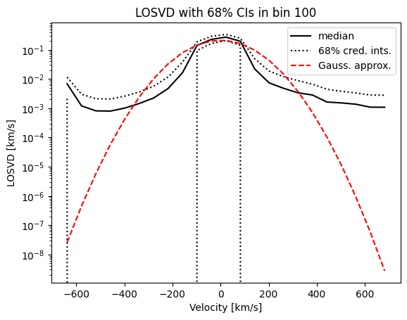
We see that BayesLOSVD does not force the LOSVD to decay at large velocities. The fat tails give rise to large standard deviations. Therefore, the sigma values in the data table are unrepresentative of the width of the main body of the distribution.
For this reason, sigma-maps for BayesLOSVD output are not recommended. By default, for BayesLOSVD kinematic maps we will only plot mean velocities. In the future, we may extend this to plot LOSVD quantiles.
Running DYNAMITE
1. Prepare the configuration file
Next prepare the DYNAMITE congfiguration file. We’ve included the file NGC4550_config.yaml in this directory. Here, we highlight a few important entries which are specific to fitting BayesLOSVD data. Firstly, we have to specify the type of the kinematics as BayesLOSVD, i.e.
system_components:
...
    stars:
        ...
        kinematics:
            sauron:
                type: BayesLOSVD
                datafile: "bayes_losvd_kins.ecsv"
                aperturefile: "aperture.dat"
                binfile: "bins.dat"
and ensure the type of the weight_solver is NNLS (since the alternative, LegacyWeightSolver is incompatible with BayesLOSVD data), i.e.
weight_solver_settings:
    type: "NNLS"
    lum_intr_rel_err: 0.01
    sb_proj_rel_err: 0.02
    nnls_solver: 'scipy'
Also, select either chi2 or kinchi2 in the configuration file’s parameter_space_settings (kinmapchi2 is incompatible with BayesLOSVD), i.e.
parameter_space_settings:
    ...
    which_chi2: "kinchi2"  # or "chi2"
    ...
Read the configuration file in,
[13]:
c = dyn.config_reader.Configuration('NGC4550_config.yaml', reset_logging=True)
[INFO] 10:57:28 - dynamite.config_reader.Configuration - Config file NGC4550_config.yaml read.
[INFO] 10:57:28 - dynamite.config_reader.Configuration - io_settings...
[INFO] 10:57:29 - dynamite.config_reader.Configuration - Output directory tree: NGC4550_output/.
[INFO] 10:57:29 - dynamite.config_reader.Configuration - system_attributes...
[INFO] 10:57:29 - dynamite.config_reader.Configuration - model_components...
[INFO] 10:57:29 - dynamite.config_reader.Configuration - system_parameters...
[INFO] 10:57:29 - dynamite.config_reader.Configuration - orblib_settings...
[INFO] 10:57:29 - dynamite.config_reader.Configuration - weight_solver_settings...
[INFO] 10:57:29 - dynamite.config_reader.Configuration - Will attempt to recover partially run models.
[INFO] 10:57:29 - dynamite.config_reader.Configuration - parameter_space_settings...
[INFO] 10:57:29 - dynamite.config_reader.Configuration - multiprocessing_settings...
[INFO] 10:57:29 - dynamite.config_reader.Configuration - ... using 4 CPUs for orbit integration.
[INFO] 10:57:29 - dynamite.config_reader.Configuration - ... using 4 CPUs for weight solving.
[INFO] 10:57:29 - dynamite.config_reader.Configuration - legacy_settings...
[INFO] 10:57:29 - dynamite.config_reader.Configuration - System assembled
[INFO] 10:57:29 - dynamite.config_reader.Settings - No value given for orblib setting quad_nr - set to its default 10.
[INFO] 10:57:29 - dynamite.config_reader.Settings - No value given for orblib setting quad_nth - set to its default 6.
[INFO] 10:57:29 - dynamite.config_reader.Settings - No value given for orblib setting quad_nph - set to its default 6.
[INFO] 10:57:29 - dynamite.config_reader.Configuration - Configuration validated
[INFO] 10:57:29 - dynamite.config_reader.Configuration - Instantiated parameter space
[INFO] 10:57:29 - dynamite.model.AllModels - Previous models have been found: Reading NGC4550_output/all_models.ecsv into AllModels.table
[INFO] 10:57:29 - dynamite.config_reader.Configuration - Instantiated AllModels object
[INFO] 10:57:29 - dynamite.model.AllModels - No all_models table update required.
2. Run the models
This will run two iterations, producing 5 models in total. It should take around 7 minutes with 4 cpus.
[14]:
# delete previous output if available
c.remove_existing_orblibs()
c.remove_existing_all_models_file(wipe_other_files=False)
c.backup_config_file(keep=3, delete_other=True)
[INFO] 10:57:29 - dynamite.config_reader.Configuration - Model output tree NGC4550_output/models/ removed.
[INFO] 10:57:29 - dynamite.config_reader.Configuration - Deleted existing NGC4550_output/all_models.ecsv.
[INFO] 10:57:29 - dynamite.model.AllModels - No previous models (file NGC4550_output/all_models.ecsv) have been found: Made an empty table in AllModels.table
[INFO] 10:57:29 - dynamite.config_reader.Configuration - Instantiated empty AllModels object
[INFO] 10:57:29 - dynamite.config_reader.Configuration - Config file backup: NGC4550_output/NGC4550_config_003.yaml.
[15]:
import time

t = time.perf_counter()

mod_iter = dyn.model_iterator.ModelIterator(config=c)

delta_t = time.perf_counter()-t
print(f'Computation time: {delta_t} seconds = {delta_t/60} minutes')
[INFO] 10:57:29 - dynamite.model_iterator.ModelIterator - LegacyGridSearch: iterations 0 and 1
[INFO] 10:57:29 - dynamite.parameter_space.LegacyGridSearch - LegacyGridSearch added 1 new model(s) out of 1
[INFO] 10:57:29 - dynamite.parameter_space.LegacyGridSearch - LegacyGridSearch added 4 new model(s) out of 4
[INFO] 10:57:29 - dynamite.model_iterator.ModelInnerIterator - ... running model 1 out of 5
[INFO] 10:57:29 - dynamite.model_iterator.ModelInnerIterator - ... running model 2 out of 5
[INFO] 10:57:29 - dynamite.model_iterator.ModelInnerIterator - ... running model 3 out of 5
[INFO] 10:57:29 - dynamite.orblib.LegacyOrbitLibrary - Calculating initial conditions
[INFO] 10:57:29 - dynamite.orblib.LegacyOrbitLibrary - Calculating initial conditions
[INFO] 10:57:29 - dynamite.orblib.LegacyOrbitLibrary - Calculating initial conditions
[INFO] 10:59:56 - dynamite.orblib.LegacyOrbitLibrary - ...done - cmd_orb_start exit code 0. Logfile: NGC4550_output/models/orblib_001_001/datfil/orbstart.log.
[INFO] 10:59:56 - dynamite.orblib.LegacyOrbitLibrary - Integrating orbit library tube orbits
[INFO] 10:59:56 - dynamite.orblib.LegacyOrbitLibrary - ...done - cmd_orb_start exit code 0. Logfile: NGC4550_output/models/orblib_000_000/datfil/orbstart.log.
[INFO] 10:59:56 - dynamite.orblib.LegacyOrbitLibrary - Integrating orbit library tube orbits
[INFO] 11:00:10 - dynamite.orblib.LegacyOrbitLibrary - ...done - cmd_tube_orbs exit code 0. Logfiles: NGC4550_output/models/orblib_001_001/datfil/orblib.log, NGC4550_output/models/orblib_001_001/datfil/triaxmass.log, NGC4550_output/models/orblib_001_001/datfil/triaxmassbin.log.
[INFO] 11:00:10 - dynamite.orblib.LegacyOrbitLibrary - Integrating orbit library box orbits
[INFO] 11:00:11 - dynamite.orblib.LegacyOrbitLibrary - ...done - cmd_tube_orbs exit code 0. Logfiles: NGC4550_output/models/orblib_000_000/datfil/orblib.log, NGC4550_output/models/orblib_000_000/datfil/triaxmass.log, NGC4550_output/models/orblib_000_000/datfil/triaxmassbin.log.
[INFO] 11:00:11 - dynamite.orblib.LegacyOrbitLibrary - Integrating orbit library box orbits
[INFO] 11:00:22 - dynamite.orblib.LegacyOrbitLibrary - ...done - cmd_box_orbs exit code 0. Logfile: NGC4550_output/models/orblib_001_001/datfil/orblibbox.log.
[INFO] 11:00:22 - dynamite.weight_solvers.NNLS - Using WeightSolver: NNLS/scipy
[INFO] 11:00:22 - dynamite.orblib.LegacyOrbitLibrary - ...done - cmd_box_orbs exit code 0. Logfile: NGC4550_output/models/orblib_000_000/datfil/orblibbox.log.
[INFO] 11:00:22 - dynamite.weight_solvers.NNLS - Using WeightSolver: NNLS/scipy
[INFO] 11:00:28 - dynamite.weight_solvers.NNLS - 'GaussHermite' kinematics required for kinmapchi2. Value set to nan.
[INFO] 11:00:28 - dynamite.weight_solvers.NNLS - NNLS problem solved and chi2 calculated.
[INFO] 11:00:28 - dynamite.config_reader.Configuration - Config file NGC4550_config.yaml copied to NGC4550_output/models/orblib_001_001/ml03.00/.
[INFO] 11:00:28 - dynamite.model_iterator.ModelInnerIterator - Model 3: NGC4550_output/models/orblib_001_001/ml03.00/model_done_staging.ecsv written.
[INFO] 11:00:29 - dynamite.weight_solvers.NNLS - 'GaussHermite' kinematics required for kinmapchi2. Value set to nan.
[INFO] 11:00:29 - dynamite.weight_solvers.NNLS - NNLS problem solved and chi2 calculated.
[INFO] 11:00:29 - dynamite.config_reader.Configuration - Config file NGC4550_config.yaml copied to NGC4550_output/models/orblib_000_000/ml03.00/.
[INFO] 11:00:29 - dynamite.model_iterator.ModelInnerIterator - Model 1: NGC4550_output/models/orblib_000_000/ml03.00/model_done_staging.ecsv written.
[INFO] 11:00:47 - dynamite.orblib.LegacyOrbitLibrary - ...done - cmd_orb_start exit code 0. Logfile: NGC4550_output/models/orblib_001_000/datfil/orbstart.log.
[INFO] 11:00:47 - dynamite.orblib.LegacyOrbitLibrary - Integrating orbit library tube orbits
[INFO] 11:01:01 - dynamite.orblib.LegacyOrbitLibrary - ...done - cmd_tube_orbs exit code 0. Logfiles: NGC4550_output/models/orblib_001_000/datfil/orblib.log, NGC4550_output/models/orblib_001_000/datfil/triaxmass.log, NGC4550_output/models/orblib_001_000/datfil/triaxmassbin.log.
[INFO] 11:01:01 - dynamite.orblib.LegacyOrbitLibrary - Integrating orbit library box orbits
[INFO] 11:01:11 - dynamite.orblib.LegacyOrbitLibrary - ...done - cmd_box_orbs exit code 0. Logfile: NGC4550_output/models/orblib_001_000/datfil/orblibbox.log.
[INFO] 11:01:11 - dynamite.weight_solvers.NNLS - Using WeightSolver: NNLS/scipy
[INFO] 11:01:17 - dynamite.weight_solvers.NNLS - 'GaussHermite' kinematics required for kinmapchi2. Value set to nan.
[INFO] 11:01:17 - dynamite.weight_solvers.NNLS - NNLS problem solved and chi2 calculated.
[INFO] 11:01:17 - dynamite.config_reader.Configuration - Config file NGC4550_config.yaml copied to NGC4550_output/models/orblib_001_000/ml03.00/.
[INFO] 11:01:17 - dynamite.model_iterator.ModelInnerIterator - Model 2: NGC4550_output/models/orblib_001_000/ml03.00/model_done_staging.ecsv written.
[INFO] 11:01:17 - dynamite.model_iterator.ModelInnerIterator - ... running model 5 out of 5
[INFO] 11:01:17 - dynamite.model_iterator.ModelInnerIterator - ... running model 4 out of 5
[INFO] 11:01:17 - dynamite.weight_solvers.NNLS - Using WeightSolver: NNLS/scipy
[INFO] 11:01:17 - dynamite.weight_solvers.NNLS - Using WeightSolver: NNLS/scipy
[INFO] 11:01:23 - dynamite.weight_solvers.NNLS - 'GaussHermite' kinematics required for kinmapchi2. Value set to nan.
[INFO] 11:01:23 - dynamite.weight_solvers.NNLS - NNLS problem solved and chi2 calculated.
[INFO] 11:01:23 - dynamite.config_reader.Configuration - Config file NGC4550_config.yaml copied to NGC4550_output/models/orblib_000_000/ml04.00/.
[INFO] 11:01:23 - dynamite.model_iterator.ModelInnerIterator - Model 5: NGC4550_output/models/orblib_000_000/ml04.00/model_done_staging.ecsv written.
[INFO] 11:01:23 - dynamite.weight_solvers.NNLS - 'GaussHermite' kinematics required for kinmapchi2. Value set to nan.
[INFO] 11:01:23 - dynamite.weight_solvers.NNLS - NNLS problem solved and chi2 calculated.
[INFO] 11:01:23 - dynamite.config_reader.Configuration - Config file NGC4550_config.yaml copied to NGC4550_output/models/orblib_000_000/ml02.00/.
[INFO] 11:01:23 - dynamite.model_iterator.ModelInnerIterator - Model 4: NGC4550_output/models/orblib_000_000/ml02.00/model_done_staging.ecsv written.
[INFO] 11:01:23 - dynamite.model_iterator.ModelInnerIterator - Iteration done, 5 model(s) calculated.
[INFO] 11:01:23 - dynamite.model_iterator.ModelInnerIterator - 5 staging file(s) deleted.
[INFO] 11:01:23 - dynamite.plotter.Plotter - kinchi2 vs. model id plot created (5 models).
[INFO] 11:01:23 - dynamite.plotter.Plotter - Plot NGC4550_output/plots/kinchi2_progress_plot.png saved in NGC4550_output/plots/
[INFO] 11:01:23 - dynamite.plotter.Plotter - Making chi2 plot scaled according to kinchi2
[INFO] 11:01:23 - dynamite.plotter.Plotter - Plot NGC4550_output/plots/kinchi2_plot.png saved in NGC4550_output/plots/
[INFO] 11:01:23 - dynamite.plotter.Plotter - Plotting kinematic maps for 1 kin_sets.
[INFO] 11:01:23 - dynamite.plotter.Plotter - Plotting kinematic maps for kin_set no 0: sauron
[INFO] 11:01:23 - dynamite.weight_solvers.NNLS - Using WeightSolver: NNLS/scipy
[INFO] 11:01:27 - dynamite.weight_solvers.NNLS - NNLS solution read from existing output
[INFO] 11:01:32 - dynamite.plotter.Plotter - Kinematic map written to NGC4550_output/plots/kinematic_map_sauron.png.
Computation time: 242.98575249602436 seconds = 4.049762541600406 minutes
Look at the summary table,
[16]:
c.all_models.table
[16]:
| m-black_hole | a-black_hole | c-dm_halo | f-dm_halo | q-stars | p-stars | u-stars | ml | chi2 | kinchi2 | kinmapchi2 | time_modified | orblib_done | weights_done | all_done | which_iter | directory |
|---|---|---|---|---|---|---|---|---|---|---|---|---|---|---|---|---|
| float64 | float64 | float64 | float64 | float64 | float64 | float64 | float64 | float64 | float64 | float64 | str256 | bool | bool | bool | int64 | str256 |
| 1000000.0 | 0.001 | 10.0 | 1.0 | 0.1 | 0.99 | 0.9999 | 3.0 | 43142.86663262113 | 4657.040278806536 | nan | 2024-12-13T09:00:29.000 | True | True | True | 0 | orblib_000_000/ml03.00/ |
| 1000000.0 | 0.001 | 10.0 | 0.31622776601683794 | 0.1 | 0.99 | 0.9999 | 3.0 | 49665.09902974907 | 4682.840221148701 | nan | 2024-12-13T09:01:17.000 | True | True | True | 1 | orblib_001_000/ml03.00/ |
| 1000000.0 | 0.001 | 10.0 | 3.1622776601683795 | 0.1 | 0.99 | 0.9999 | 3.0 | 41678.77123172247 | 4661.308745747497 | nan | 2024-12-13T09:00:28.000 | True | True | True | 1 | orblib_001_001/ml03.00/ |
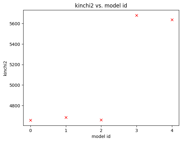
| 1000000.0 | 0.001 | 10.0 | 1.0 | 0.1 | 0.99 | 0.9999 | 2.0 | 44184.754413096074 | 5680.738415615588 | nan | 2024-12-13T09:01:23.000 | True | True | True | 1 | orblib_000_000/ml02.00/ |
| 1000000.0 | 0.001 | 10.0 | 1.0 | 0.1 | 0.99 | 0.9999 | 4.0 | 44133.84076002365 | 5637.300173398443 | nan | 2024-12-13T09:01:23.000 | True | True | True | 1 | orblib_000_000/ml04.00/ |
3. Look at plots of the results
Some plots have been automatically created as the models were run, stored in the directory NGC4550_output/plots/. Let’s look at some. After running the example above, you should find versions of the following plots at the locations below.
Kinematic map
NGC4550_output/plots/kinematic_map_sauron.png
We can also obtain the plot directly from the model iterator’s get_plots() method (the kinematics are the return value’s third element),
[17]:
kinmap = mod_iter.get_plots()[2]
print('First (and only) kinematics: ' + kinmap[0][1])  # The name of the kinematics
kinmap[0][0]  # The plot
First (and only) kinematics: sauron
[17]:
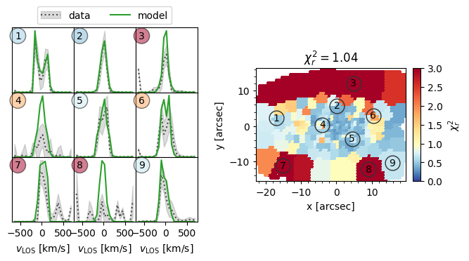
The right half shows a map of the reduced chi2 of the best fitting orbit-based model to the observed LOSVD. The left half shows nine examples, which have been chosen to span the variety in the observed kinematics. We see that in some locations (e.g. 1, 2, 5, 9) the observed LOSVD is fit well, however in many others it is not. In particular, some bins (e.g. 7, 8) have very spiky observed LOSVDs while others (e.g. 3, 6) have peaks at the most negative velocitites which is most likely an artifact.
Chi2 evolution
NGC4550_output/plots/kinchi2_progress_plot.png
[18]:
mod_iter.get_plots()[0]
[18]:
Chi2 distribution against model parameters
NGC4550_output/plots/kinchi2_plot.png
[19]:
mod_iter.get_plots()[1]
[19]:
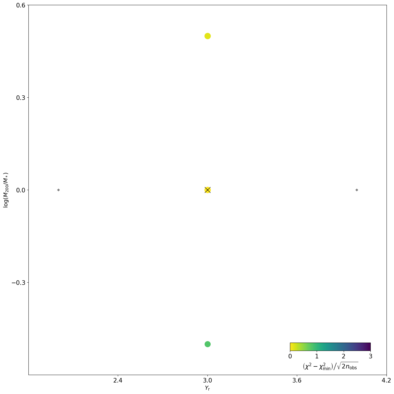
In this case only two parameters have been left free, and only a small handful of models have been evaluated. As more models explore more of parameter space, this plot will begin to look more interesting!
