Note:
This page was generated from a Jupyter notebook which can be found at
docs/tutorial_notebooks/8_coloring.ipynb
in your DYNAMITE directory.
—-
8. Coloring - BETA -
This notebook takes a look at coloring (fitting population data). Upon its first start, it will create a model for the example galaxy FCC167. Based on that model and observational data, the notebook will fit age and metallicity of the populations.
Please note that this notebook is still in beta, as is the DYNAMITE coloring functionality. For more information on the options and functionality of the methods described here, please refer to the API docs.
8.1. Prerequisites
Import the required modules.
[1]:
import numpy as np
import matplotlib.pyplot as plt
import pymc as pm  # only necessary for posterior plots
from vorbin.voronoi_2d_binning import voronoi_2d_binning
import dynamite as dyn

print('DYNAMITE version', dyn.__version__)
# print('    installed at ', dyn.__path__)  # Uncomment to print the complete DYNAMITE installation path
/var/folders/1b/fphkt4y96ssbkc0ssnj56m1c0000gn/T/ipykernel_8132/2984419256.py:4: UserWarning: ⚠️ VorBin is deprecated and superseded by PowerBin https://pypi.org/project/powerbin/
  from vorbin.voronoi_2d_binning import voronoi_2d_binning
DYNAMITE version 5.0.0
Run the DYNAMITE model. The configuration file FCC167_config.yaml fixes all parameter to a specific value, resulting in a single model. For performance, the orbit library is rather small, so the calculation time should only take a few minutes. Note that the model will not be run if already existing on the disk (e.g., if the notebook is re-run).
[2]:
fname = 'FCC167_config.yaml'
c = dyn.config_reader.Configuration(fname, reset_logging=True)
# c = dyn.config_reader.Configuration(fname, reset_logging=True, reset_existing_output=True)  # uncomment to force fresh run
_ = dyn.model_iterator.ModelIterator(c)
[INFO] 16:12:28 - dynamite.config_reader.Configuration - Config file FCC167_config.yaml read.
[INFO] 16:12:28 - dynamite.config_reader.Configuration - io_settings...
[INFO] 16:12:28 - dynamite.config_reader.Configuration - Output directory tree: FCC167_output/.
[INFO] 16:12:28 - dynamite.config_reader.Configuration - system_attributes...
[INFO] 16:12:28 - dynamite.config_reader.Configuration - model_components...
[WARNING] 16:12:28 - dynamite.config_reader.Configuration - Component bh: the attribute contributes_to_potential is DEPRECATED and will be ignored. In a future DYNAMITE release this will cause an error.
[WARNING] 16:12:28 - dynamite.config_reader.Configuration - Component dh: the attribute contributes_to_potential is DEPRECATED and will be ignored. In a future DYNAMITE release this will cause an error.
[WARNING] 16:12:28 - dynamite.config_reader.Configuration - Component stars: the attribute contributes_to_potential is DEPRECATED and will be ignored. In a future DYNAMITE release this will cause an error.
[INFO] 16:12:28 - dynamite.config_reader.Configuration - system_parameters...
[INFO] 16:12:28 - dynamite.config_reader.Configuration - orblib_settings...
[INFO] 16:12:28 - dynamite.config_reader.Configuration - weight_solver_settings...
[INFO] 16:12:28 - dynamite.config_reader.Configuration - Will attempt to recover partially run models.
[INFO] 16:12:28 - dynamite.config_reader.Configuration - parameter_space_settings...
[INFO] 16:12:28 - dynamite.config_reader.Configuration - legacy_settings...
[INFO] 16:12:28 - dynamite.config_reader.Configuration - multiprocessing_settings...
[INFO] 16:12:28 - dynamite.config_reader.Configuration - ... using 8 CPUs for orbit integration.
[INFO] 16:12:28 - dynamite.config_reader.Configuration - ... using 8 CPUs for ncpus_weights.
[INFO] 16:12:28 - dynamite.config_reader.Configuration - ... using 8 CPUs for ncpus_ext.
[INFO] 16:12:28 - dynamite.config_reader.Configuration - System assembled
[INFO] 16:12:28 - dynamite.config_reader.Configuration - Configuration validated
[INFO] 16:12:28 - dynamite.config_reader.Configuration - Instantiated parameter space
[INFO] 16:12:28 - dynamite.model.AllModels - Previous models have been found: Reading FCC167_output/all_models.ecsv into AllModels.table
[INFO] 16:12:28 - dynamite.config_reader.Configuration - Instantiated AllModels object
[INFO] 16:12:28 - dynamite.model.AllModels - No all_models table update required.
[INFO] 16:12:28 - dynamite.model_iterator.ModelIterator - LegacyGridSearch: iteration 1
[INFO] 16:12:28 - dynamite.parameter_space.LegacyGridSearch - LegacyGridSearch added 0 new model(s) out of 0
[INFO] 16:12:28 - dynamite.model_iterator.ModelIterator - Stopping after iteration 1 because {'stop': True, 'n_max_mods_reached': False, 'n_max_iter_reached': False, 'min_delta_chi2_reached': False, 'n_new_models': 0, 'last_iter_added_no_new_models': True}.
8.2. Voronoi phase space binning
The model’s orbits in the phase space of circularity \(\lambda_z\) versus time-averaged orbital radius \(r\) are binned into \(N_\mathrm{bundle}\) Voronoi orbit bundles. Each Voronoi orbit bundle amounts to a certain minimum total weight.
First, we need to choose the underlying resolution in \(r\) and \(\lambda_z\):
[3]:
# Number of desired r and lambda_z bins
nr = 6  # 20
nl = 7  # 41
Optional step: Before binning the orbits, let’s have a look at the \(r\) - \(\lambda_z\) phase space. The standard DYNAMITE orbit distribution plot with the parameter force_lambda_z=True will plot the distribution of all orbits. Note that the plot title is incorrect (all orbits are included in the plot, not only the short axis tubes).
[4]:
plotter = dyn.plotter.Plotter(c)
[5]:
# NOTE: when using force_lambda_z=True, then the title of the orbit-distribution plot is incorrect: all orbits are shown in this distribution - not only short-axis tubes!
#       If force_lambda_z is True, then the entire orbit distribution is collapsed onto (r, lambda_z) space.
#       This is done by forcing all orbits to be classified as short axis-tube orbits.
fig2 = plotter.orbit_distribution(model=None,
                                  minr=None,
                                  maxr=None,
                                  r_scale='linear',
                                  nr=nr,
                                  nl=nl,
                                  orientation='vertical',
                                  subset='short',
                                  force_lambda_z=True)
[INFO] 16:12:28 - dynamite.orblib.LegacyOrbitLibrary - Orbit library classification:
[INFO] 16:12:28 - dynamite.orblib.LegacyOrbitLibrary -     - 0.0% box
[INFO] 16:12:28 - dynamite.orblib.LegacyOrbitLibrary -     - 0.0% x-tubes
[INFO] 16:12:28 - dynamite.orblib.LegacyOrbitLibrary -     - 0.0% y-tubes
[INFO] 16:12:28 - dynamite.orblib.LegacyOrbitLibrary -     - 100.0% z-tubes
[INFO] 16:12:28 - dynamite.orblib.LegacyOrbitLibrary -     - 0.0% other types
[INFO] 16:12:28 - dynamite.orblib.LegacyOrbitLibrary - Amongst tubes, % with only one nonzero component of L:
[INFO] 16:12:28 - dynamite.orblib.LegacyOrbitLibrary -     - 0.0% of x-tubes
[INFO] 16:12:28 - dynamite.orblib.LegacyOrbitLibrary -     - 0.0% of y-tubes
[INFO] 16:12:28 - dynamite.orblib.LegacyOrbitLibrary -     - 43.1% of z-tubes
[INFO] 16:12:28 - dynamite.orblib.LegacyOrbitLibrary - Orbit library classification DONE.
[INFO] 16:12:29 - dynamite.weight_solvers.NNLS - Using WeightSolver: NNLS/scipy
[INFO] 16:12:29 - dynamite.weight_solvers.NNLS - NNLS solution read from existing output FCC167_output/models/orblib_000_000/ml05.40/orbit_weights.ecsv.
[INFO] 16:12:29 - dynamite.plotter.Plotter - Plotting orbit distribution for orbit classes short: 1 subplot(s).
[INFO] 16:12:29 - dynamite.plotter.Plotter - fig_size=3.75.
[INFO] 16:12:29 - dynamite.plotter.Plotter - Plot FCC167_output/plots/orbit_distribution.png saved.

The Voronoi binning of orbits in the radius-circularity phase space is done by a method in the dyn.coloring.Coloring class:
[6]:
coloring = dyn.coloring.Coloring(c, nr=nr, nl=nl)
[INFO] 16:12:29 - dynamite.coloring.Coloring - Coloring initialized with minr=0.0 kpc, maxr=12.066484820700378 kpc, nr=6, nl=7.
The original n_orbits orbit bundles are binned into fewer \(N_\mathrm{bundle}=\)n_bundle Voronoi orbit bundles with each of these Voronoi bundles accounting for a weight of at least vor_weight.
[7]:
vor_weight = 0.05 # define the desired (minimum) total orbital weight in each Voronoi bin
The method coloring.bin_phase_space() performs the binning of orbits, based on the best-fitting model so far (in our case this is the only model). The result of the binning is a tuple (vor_bundle_mapping, phase_space_binning):
vor_bundle_mapping :    np.array of shape (n_bundle, n_orbits)
                        Mapping between the "original" orbit bundles and the Voronoi
                        orbit bundles: vor_bundle_mapping(i_bundle, i_orbit) is the
                        fraction of i_orbit assigned to i_bundle, multiplied by i_orbit's weight.
phase_space_binning :   dict
                        'out':  np.array of shape (3, n_bundle), the Voronoi binning output:
                                weighted Voronoi bin centroid coordinates r_bar, lambda_bar
                                and Voronoi bin total weights
                        'map':  np.array of shape (nr*nl,) the phase space mapping:
                                Voronoi bin numbers for each input bin
As the binning can be time-consuming, coloring.bin_phase_space() will write the binning result to the model directory so that subsequent calls with the same parameters for the same model will read the existing binning from disk if use_cache=True.
[8]:
vor_bundle_mapping, phase_space_binning = coloring.bin_phase_space(model=None,
                                                                   vor_weight=vor_weight,
                                                                   vor_ignore_zeros=True,
                                                                   make_diagnostic_plots=True,
                                                                   extra_diagnostic_output=True,
                                                                   cvt=False,
                                                                   wvt=False,
                                                                   use_noise=True,
                                                                   use_cache=False)  # set use_cache=False to force fresh binning
[INFO] 16:12:29 - dynamite.orblib.LegacyOrbitLibrary - Orbit library classification:
[INFO] 16:12:29 - dynamite.orblib.LegacyOrbitLibrary -     - 0.0% box
[INFO] 16:12:29 - dynamite.orblib.LegacyOrbitLibrary -     - 0.0% x-tubes
[INFO] 16:12:29 - dynamite.orblib.LegacyOrbitLibrary -     - 0.0% y-tubes
[INFO] 16:12:29 - dynamite.orblib.LegacyOrbitLibrary -     - 100.0% z-tubes
[INFO] 16:12:29 - dynamite.orblib.LegacyOrbitLibrary -     - 0.0% other types
[INFO] 16:12:29 - dynamite.orblib.LegacyOrbitLibrary - Amongst tubes, % with only one nonzero component of L:
[INFO] 16:12:29 - dynamite.orblib.LegacyOrbitLibrary -     - 0.0% of x-tubes
[INFO] 16:12:29 - dynamite.orblib.LegacyOrbitLibrary -     - 0.0% of y-tubes
[INFO] 16:12:29 - dynamite.orblib.LegacyOrbitLibrary -     - 43.1% of z-tubes
[INFO] 16:12:29 - dynamite.orblib.LegacyOrbitLibrary - Orbit library classification DONE.
[INFO] 16:12:31 - dynamite.weight_solvers.NNLS - Using WeightSolver: NNLS/scipy
[INFO] 16:12:31 - dynamite.weight_solvers.NNLS - NNLS solution read from existing output FCC167_output/models/orblib_000_000/ml05.40/orbit_weights.ecsv.
[WARNING] 16:12:31 - dynamite.coloring.Coloring - The total circularity of the orbit distribution is negative (lambda_z=-0.2638585329255835), flipping the sign of lambda_z. Beware of side effects! Hint: consider changing the position angle in the aperture file by ±180 degrees.
/Users/user/.local/lib/python3.11/site-packages/dynamite/coloring.py:298: UserWarning: ⚠️ VorBin is deprecated and superseded by PowerBin https://pypi.org/project/powerbin/
  voronoi_2d_binning(*vor_in,
[INFO] 16:12:32 - dynamite.coloring.Coloring - 360 original orbit bundles aggregated into 11 Voronoi bundles.
[INFO] 16:12:32 - dynamite.coloring.Coloring - Voronoi binning metadata read from FCC167_output/models/orblib_000_000/ml05.40/voronoi_orbit_bundles.yaml.
[INFO] 16:12:32 - dynamite.coloring.Coloring - Voronoi binning metadata exists, will overwrite bundle data.
[INFO] 16:12:32 - dynamite.coloring.Coloring - Voronoi orbit bundle mapping saved in FCC167_output/models/orblib_000_000/ml05.40/voronoi_orbit_bundles_000.npz.
Bin-accretion...
14  initial bins.
Reassign bad bins...
11  good bins.
Unbinned pixels: 4/20
Fractional S/N scatter (per cent): 27.10
Elapsed time accretion: 0.01 seconds
Elapsed time optimization: 0.00 seconds


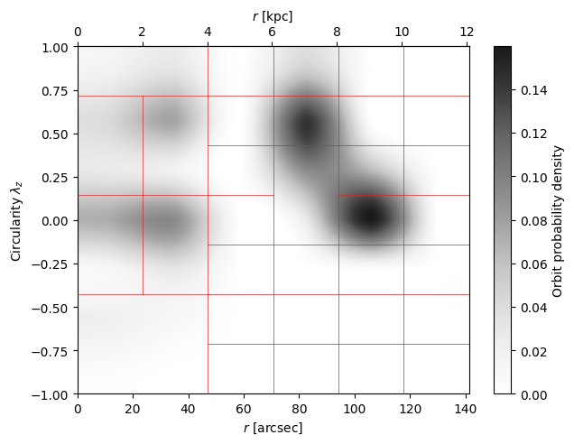
Let’s visualize the Voronoi bundle mapping, starting with the probability density of stellar orbits in the circularity-radius phase space, overlayed by the Voronoi binning scheme:
[9]:
coloring.orbit_bundle_plot(phase_space_mapping=phase_space_binning['map']);
[INFO] 16:12:33 - dynamite.coloring.Coloring - Creating orbit bundle plot.
[INFO] 16:12:33 - dynamite.coloring.Coloring - No orbit distribution provided, calculating from model parameter.
[INFO] 16:12:33 - dynamite.orblib.LegacyOrbitLibrary - Orbit library classification:
[INFO] 16:12:33 - dynamite.orblib.LegacyOrbitLibrary -     - 0.0% box
[INFO] 16:12:33 - dynamite.orblib.LegacyOrbitLibrary -     - 0.0% x-tubes
[INFO] 16:12:33 - dynamite.orblib.LegacyOrbitLibrary -     - 0.0% y-tubes
[INFO] 16:12:33 - dynamite.orblib.LegacyOrbitLibrary -     - 100.0% z-tubes
[INFO] 16:12:33 - dynamite.orblib.LegacyOrbitLibrary -     - 0.0% other types
[INFO] 16:12:33 - dynamite.orblib.LegacyOrbitLibrary - Amongst tubes, % with only one nonzero component of L:
[INFO] 16:12:33 - dynamite.orblib.LegacyOrbitLibrary -     - 0.0% of x-tubes
[INFO] 16:12:33 - dynamite.orblib.LegacyOrbitLibrary -     - 0.0% of y-tubes
[INFO] 16:12:33 - dynamite.orblib.LegacyOrbitLibrary -     - 43.1% of z-tubes
[INFO] 16:12:33 - dynamite.orblib.LegacyOrbitLibrary - Orbit library classification DONE.
[INFO] 16:12:33 - dynamite.weight_solvers.NNLS - Using WeightSolver: NNLS/scipy
[INFO] 16:12:33 - dynamite.weight_solvers.NNLS - NNLS solution read from existing output FCC167_output/models/orblib_000_000/ml05.40/orbit_weights.ecsv.
[WARNING] 16:12:33 - dynamite.coloring.Coloring - The total circularity of the orbit distribution is negative (lambda_z=-0.2638585329255835), flipping the sign of lambda_z. Beware of side effects! Hint: consider changing the position angle in the aperture file by ±180 degrees.
[WARNING] 16:12:33 - dynamite.coloring.Coloring - Cannot properly plot Voronoi binning containing NaNs currently.
[INFO] 16:12:33 - dynamite.coloring.Coloring - Orbit bundle plot saved in FCC167_output/plots/orbit_bundle_plot.png.
As a quick check, let’s plot the orbit weights in each \((r, \lambda_z)\) Voronoi bin. Note that most likely the exact desired weight of the Voronoi bins will not be met, especially for small orbit libraries.
[10]:
plt.bar([str(i) for i in range(phase_space_binning['out'].shape[1])], phase_space_binning['out'][2])
plt.xlabel('Voronoi bin ID')
plt.ylabel('Weight')
plt.show()

Now, let’s visualize how much weight each original orbit bundle contributes to each Voronoi orbit bundle.
Original orbit bundles with zero weight in the specific model will not contribute to any of the Voronoi orbit bundles.
Each original orbit bundle consists of one actual orbit if
dithering=1in the configuration file’sorblib_settings, but will comprise multiple orbits ifdithering > 1. In the latter case, one original orbit bundle can be split among neighboring bins in the radius-circularity phase space and can hence contribut to multiple (neighboring) Voronoi orbit bundles.
[11]:
plt.figure(figsize=(24,4))
plt.gca().set_title('Weight that each orbit bundle contributes to Voronoi orbit bundles')
bundle_map = np.copy(vor_bundle_mapping)
bundle_map[bundle_map == 0] = np.nan
plt.pcolormesh(np.log10(bundle_map, where=bundle_map is not np.nan), shading='flat', cmap='Greys')
plt.xlabel('Original orbit bundle id')
plt.ylabel('Voronoi orbit bundle id')
plt.colorbar(label='log Weight')
[11]:
<matplotlib.colorbar.Colorbar at 0x124ce0450>

For the subsequent analysis, we will need to know how much mass (for mass-weighted models) or flux (for light-weighted models) each Voronoi orbit bundle contributes to each spatial bin. As the concept of orbit bundles per se is independent of coloring (fitting population data), the associated method is part of the dyn.analysis.Analysis class:
[12]:
a = dyn.analysis.Analysis(c) # orbit bundle maps are residing in the Analysis class
The method get_orbit_bundle_maps() returns an astropy table with as many rows as there are spatial bins and the number of columns is the number of Voronoi orbit bundles plus 1: Each Voronoi orbit bundle’s contribution corresponds to one column and at the end there is the combined bundle’s contribution in column ‘flux_all’.
Setting the parameter create_figure=True will create a figure of the individual orbit bundles’ contributions and return it along with the bundle maps (see the commented-out example below - try it…). Setting normalize=True will normalize the mass (flux) contributions so that in each spatial bin the sum of all orbit bundles’ contributions is 1. We activate this option because we will need normalized flux in the Bayesian statistical analysis further down.
[13]:
# bundle_maps, bundle_figure = a.get_orbit_bundle_maps(pop_set=0,
#                                                      bundle_mapping=vor_bundle_mapping,
#                                                      normalize=True,
#                                                      create_figure=True)  # comment-in to view the plots
bundle_maps = a.get_orbit_bundle_maps(pop_set=0,
                                      bundle_mapping=vor_bundle_mapping,
                                      normalize=True,
                                      create_figure=False)  # calculation only, won't display the plots
[INFO] 16:12:33 - dynamite.analysis.Analysis - Getting model projected masses.
[INFO] 16:12:33 - dynamite.weight_solvers.NNLS - Using WeightSolver: NNLS/scipy
[INFO] 16:12:33 - dynamite.weight_solvers.NNLS - NNLS solution read from existing output FCC167_output/models/orblib_000_000/ml05.40/orbit_weights.ecsv.
[14]:
print(f'{type(bundle_maps) = }\n{len(bundle_maps) = }\n{bundle_maps.colnames = }')
type(bundle_maps) = <class 'astropy.table.table.Table'>
len(bundle_maps) = 974
bundle_maps.colnames = ['flux_000', 'flux_001', 'flux_002', 'flux_003', 'flux_004', 'flux_005', 'flux_006', 'flux_007', 'flux_008', 'flux_009', 'flux_010', 'flux_all']
As you see, the bundle_maps contain the Voronoi orbit bundles’ contributions along with the aggregate map. For the subsequent calculations, we will only need the data in columns corresponding to the individual Voronoi bundles which we store in flux_data_norm:
[15]:
flux_data_norm = np.array([bundle_maps[a] for a in bundle_maps.columns if a != 'flux_all']).T
print(f'{flux_data_norm.shape = }') # (n_spatial_bins, n_bundle)
flux_data_norm.shape = (974, 11)
8.3. Bayesian statistical analysis
Fitting age and metallicity essentially follows the procedure described in Zhu et al., 2020, MNRAS, 496, 1579. For brevity, only the priors “R1” for both age and metallicity will be used. In the following sections, equation numbers refer to the corresponding equations in that paper.
The fitting is done via Bayesian inference as provided by the Python package PyMC. The model uses a truncated normal or lognormal distribution for the prior of the observed quantity and a Student’s t distribution with fixed \(\sigma\) (Half-Cauchy distributed with \(\beta=5\)) and \(\nu\) (Exponential distributed with parameter 1/30) parameters for the likelihood of the observed data. The solution method uses the Markov chain Monte Carlo (MCMC) sampling algorithm NUTS (No-U-Turn Sampler), initialized with the ADVI(Automatic Differentiation Variational Inference) method.
There is no need to directly interact with PyMC. DYNAMITE users can call the coloring.fit_bayesian() method that has many settings predefined already (see below).
The chain is initialized with the ADVI (automatic differentiation variational inference) with 200000 draws and 2500 tuning steps. The last 500 MCMC steps are used to get the mean and standard deviation of the age and metallicity, respectively:
[16]:
sample = {'n_draws': 500,
          'n_tune': 2500,
          'advi_init': 200000}
Finally, we need to assign some DYNAMITE data structures (note that currently, we only support one population dataset stars.population_data[0]):
[17]:
stars = c.system.get_unique_triaxial_visible_component()
pops = stars.population_data[0]
age, dage, met, dmet = [pops.get_data()[i] for i in ('age', 'dage', 'met', 'dmet')]  # dage and dmet will not be used
8.3.1. Age
The age prior is a bounded normal distribution \(f(t_k|\mu_k,\sigma_k)\) with a lower boundary of 0, an upper boundary of 20, and \(\mu_k=\mathrm{Randn}(<t_\mathrm{obs}>,2\sigma(t_\mathrm{obs}))\) and \(\sigma_k=2\sigma(t_\mathrm{obs})\), see Eq. (11)-(13):
[18]:
prior_t = {'mu': np.random.normal(age.mean(), 2 * age.std(), size=len(vor_bundle_mapping)),  # Eq. (12)
           'sigma': 2 * age.std(),                                                           # Eq. (13)
           'lower': 0,
           'upper': 20}
[19]:
model_t, trace_t = coloring.fit_bayesian(prior_dist='normal',
                                         prior_par=prior_t,
                                         flux_data_norm=flux_data_norm,
                                         obs_data=age,
                                         sample=sample)
[INFO] 16:12:34 - dynamite.coloring.Coloring - Fitting Bayesian model to the observed data.
Initializing NUTS using advi...
/Users/user/.local/lib/python3.11/site-packages/rich/live.py:256: UserWarning: install "ipywidgets" for Jupyter
support
  warnings.warn('install "ipywidgets" for Jupyter support')
Convergence achieved at 24800
Interrupted at 24,799 [12%]: Average Loss = 1,259.4
Multiprocess sampling (4 chains in 4 jobs)
NUTS: [pop, student_t_sigma, student_t_nu]
/Users/user/.local/lib/python3.11/site-packages/rich/live.py:256: UserWarning: install "ipywidgets" for Jupyter
support
  warnings.warn('install "ipywidgets" for Jupyter support')
Sampling 4 chains for 2_500 tune and 500 draw iterations (10_000 + 2_000 draws total) took 30 seconds.
The effective sample size per chain is smaller than 100 for some parameters.  A higher number is needed for reliable rhat and ess computation. See https://arxiv.org/abs/1903.08008 for details
[INFO] 16:13:18 - dynamite.coloring.Coloring - Bayesian model fitting completed. Shape of posterior: (n_chain, n_draw, n_dim_0) = (4, 500, 11).
Optional: inspect the Bayesian model details via
[20]:
model_t
[20]:
Note that per default PyMC per default uses as many chains as there are physical CPU cores available (e.g., 4). There are 3000 draws in each chain, corresponding to 2500 tuning steps and 500 draws for the results.
The resulting age values are accessible via trace_t.posterior['pop']:
[21]:
trace_t.posterior['pop']
[21]:
<xarray.DataArray 'pop' (chain: 4, draw: 500, pop_dim_0: 11)> Size: 176kB
array([[[12.89962527,  8.87668501, 15.64019117, ..., 12.20887756,
         13.41218409, 17.11359381],
        [11.37556384,  8.62920645, 15.38633826, ..., 12.45954738,
         13.25332828, 16.81006188],
        [11.39833081,  9.06397144, 14.22226738, ..., 12.14612488,
         13.57737922, 16.59497595],
        ...,
        [10.91381665,  9.35372588, 14.87542356, ..., 11.26148723,
         13.55417847, 19.20162142],
        [11.99676186,  9.42115083, 16.67124461, ..., 11.23265897,
         13.73311946, 18.90073488],
        [12.15617143,  9.7704746 , 16.55425955, ..., 11.52052676,
         13.5478017 , 18.94260724]],

       [[10.60072594, 10.21439012, 17.43473256, ..., 11.69797587,
         13.4708967 , 18.2705939 ],
        [10.93494307, 10.00359603, 17.74228426, ..., 11.5500025 ,
         13.67598177, 18.07868708],
        [10.15329261, 11.76390033, 17.36100088, ..., 11.53859266,
         13.59391702, 17.94922114],
...
        [11.80770885,  8.00681104, 16.09075484, ..., 12.61018805,
         13.35206806, 16.53983573],
        [12.1466318 ,  9.21928934, 16.1027809 , ..., 11.84660473,
         13.56176189, 17.36675891],
        [10.96730382,  9.76452694, 17.54357947, ..., 12.04058517,
         13.41816417, 17.96242408]],

       [[12.25444977,  8.36752154, 17.41300026, ..., 11.63931373,
         13.50687269, 18.41679035],
        [11.16107569,  8.89108367, 15.69099886, ..., 11.89163801,
         13.58857712, 17.78486379],
        [11.65100793,  8.90008467, 16.30720569, ..., 11.3471518 ,
         13.62908659, 18.80946583],
        ...,
        [11.78792546,  8.48491595, 16.97857456, ..., 12.19194904,
         13.09771117, 18.14902482],
        [12.32344511,  9.27541683, 16.51224193, ..., 11.83119875,
         13.47837135, 17.92722692],
        [12.29005969,  6.62892537, 16.46394751, ..., 11.69926317,
         13.7852588 , 17.64701651]]])
Coordinates:
  * chain      (chain) int64 32B 0 1 2 3
  * draw       (draw) int64 4kB 0 1 2 3 4 5 6 7 ... 493 494 495 496 497 498 499
* pop_dim_0 (pop_dim_0) int64 88B 0 1 2 3 4 5 6 7 8 9 10We store it in symbol age_posterior for later. It is a data structure compatible with an array of shape (< number of chains >, < number of draws >, <\(N_\mathrm{bundle}\)>). Consequently, the mean and error of each Voronoi orbit bundle’s age are given by age_mean = age_posterior.mean(axis=(0,1)) and age_err = age_posterior.std(axis=(0,1)), respectively:
[22]:
age_posterior = trace_t.posterior['pop']
age_mean = age_posterior.mean(axis=(0,1))
age_err = age_posterior.std(axis=(0,1))
[23]:
age_mean
[23]:
<xarray.DataArray 'pop' (pop_dim_0: 11)> Size: 88B
array([11.57744221,  9.11086204, 16.50716612, 10.57703798,  6.6933375 ,
       12.20259199, 13.91483769, 12.21230502, 11.66748668, 13.59304705,
       18.02722331])
Coordinates: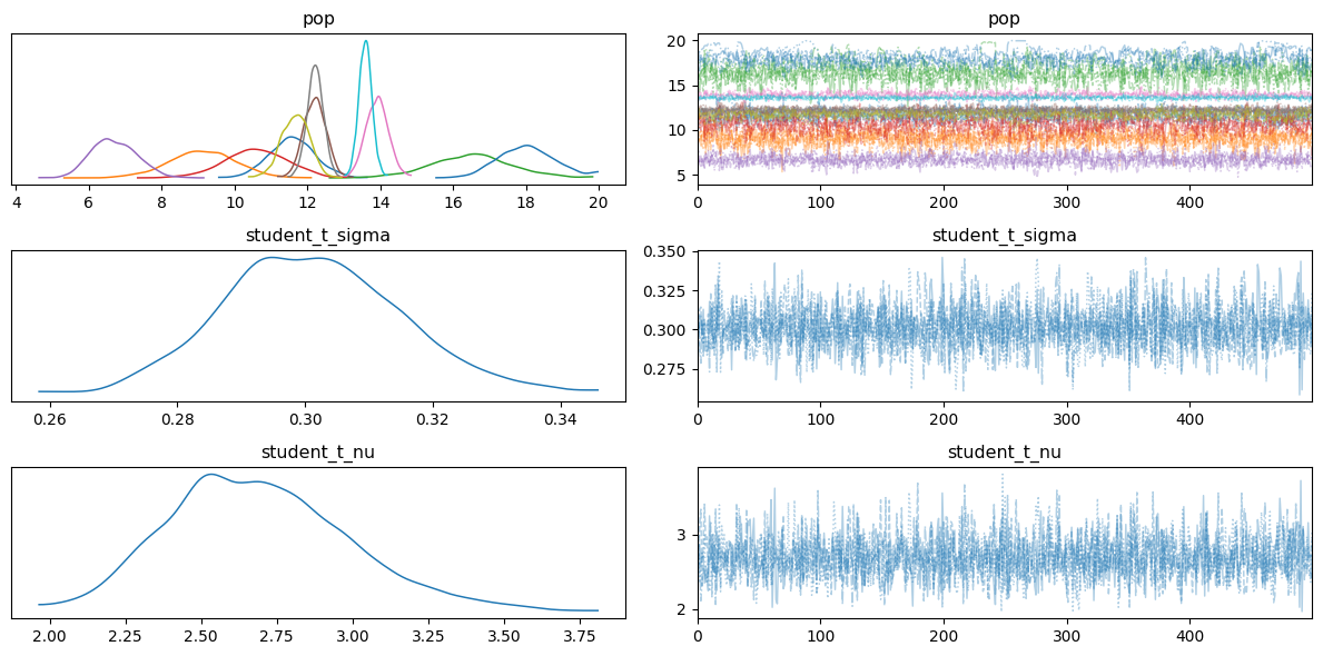
* pop_dim_0 (pop_dim_0) int64 88B 0 1 2 3 4 5 6 7 8 9 10Optional: display the posterior plot (requires the PyMC module to be imported). To better format the figure, we use tight_layout(), but as plot_trace() returns an array of Axes objects, we first must extract the figure:
[24]:
axes_array = pm.plot_trace(trace_t, combined=True)
figure = axes_array[0,0].figure
figure.tight_layout()
8.3.2. Metallicity
The metallicity prior is a bounded lognormal distribution \(f(Z_k|\mu_k,\sigma_k)\) with a lower boundary of 0, an upper boundary of 10, and \(\mu_k=\ln(\mathrm{Randn}(<Z_\mathrm{obs}>,\sigma(Z_\mathrm{obs})))\) and \(\sigma_k=\sigma(Z_\mathrm{obs})\), see Eq. (16)-(18):
[25]:
prior_z = {'mu': np.log(np.random.normal(met.mean(), met.std(), size=len(vor_bundle_mapping))),  # (17)
           'sigma': met.std(),  # (18)
           'lower': 0,
           'upper': 10}
[26]:
model_z, trace_z = coloring.fit_bayesian(prior_dist='lognormal',
                                         prior_par=prior_z,
                                         flux_data_norm=flux_data_norm,
                                         obs_data=met,
                                         sample=sample)
[INFO] 16:13:20 - dynamite.coloring.Coloring - Fitting Bayesian model to the observed data.
Initializing NUTS using advi...
/Users/user/.local/lib/python3.11/site-packages/rich/live.py:256: UserWarning: install "ipywidgets" for Jupyter
support
  warnings.warn('install "ipywidgets" for Jupyter support')
Convergence achieved at 16000
Interrupted at 15,999 [7%]: Average Loss = 592.29
Multiprocess sampling (4 chains in 4 jobs)
NUTS: [pop, student_t_sigma, student_t_nu]
/Users/user/.local/lib/python3.11/site-packages/rich/live.py:256: UserWarning: install "ipywidgets" for Jupyter
support
  warnings.warn('install "ipywidgets" for Jupyter support')
Sampling 4 chains for 2_500 tune and 500 draw iterations (10_000 + 2_000 draws total) took 27 seconds.
[INFO] 16:13:54 - dynamite.coloring.Coloring - Bayesian model fitting completed. Shape of posterior: (n_chain, n_draw, n_dim_0) = (4, 500, 11).
Optional: inspect the Bayesian model details via
[27]:
model_z
[27]:
In analogy to above, the resulting metallicity values are accessible via trace_z.posterior['pop'], a data structure compatible with an array of shape (< number of chains >, < number of draws >, <\(N_\mathrm{bundle}\)>). After storing it in met_posterior, the mean and error of each Voronoi orbit bundle’s metallicity are given by met_mean = met_posterior.mean(axis=(0,1)) and met_err = met_posterior.std(axis=(0,1)), respectively:
[28]:
met_posterior = trace_z.posterior['pop']
met_mean = met_posterior.mean(axis=(0,1))
met_err = met_posterior.std(axis=(0,1))
Optional: display the posterior plot (requires the PyMC module to be imported):
[29]:
axes_array = pm.plot_trace(trace_z, combined=True)
figure = axes_array[0,0].figure
figure.tight_layout()

8.4. Results
8.4.1. Check how the model matches the data
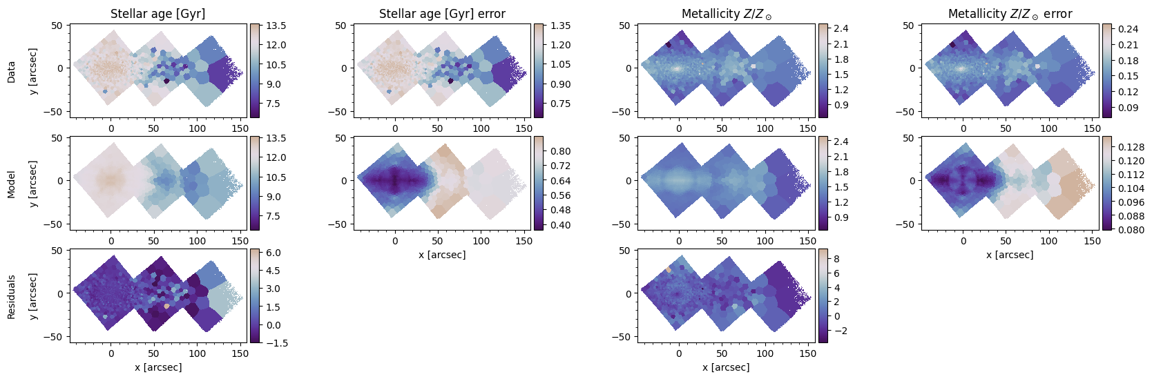
Here, we plot the observed age and metallicity maps along with the maps of the fitted age and metallicity data. Note that for the observed data (first row), the errors refer to the read-in observation errors and for the fitted data (second row), the error columns refer to the standard deviations of the posteriors for age and metallicity, respectively. The population maps are consistent with those used in the kinematic map plots. Also, the residuals are defined as
residual = (model - data) / data_error, consistent with the kinematic maps.
[30]:
coloring.pop_maps(pop_data={'age': 'Stellar age [Gyr]', 'met': r'Metallicity $Z/Z_\odot$'},  # choose the population datasets to be plotted
                  model_data=[age_mean, age_err, met_mean, met_err],                         # calculated from the posteriors
                  flux_norm=flux_data_norm,                                                  # resulting from get_orbit_bundle_maps() above
                  cbar_lims='data');                                                         # 'data', 'model', or 'auto'
[INFO] 16:13:55 - dynamite.coloring.Coloring - Population data maps: plotting data and errors for 2 population datasets: ['age', 'met'].
[INFO] 16:13:58 - dynamite.coloring.Coloring - Population data maps saved in FCC167_output/plots/population_maps.png.
Including the error columns is optional. In the function call above, model_data has twice the number of entries in pop_data, which results in every other column in pop_data being interpreted as the error of the preceding dataset. If model_data and pop_data have the same lengths, just the datasets, but no errors are plotted:
[31]:
coloring.pop_maps(pop_data={'age': 'Stellar age [Gyr]', 'met': r'Metallicity $Z/Z_\odot$'},
                  model_data=[age_mean, met_mean],
                  flux_norm=flux_data_norm,
                  cbar_lims='data');
[INFO] 16:14:02 - dynamite.coloring.Coloring - Population data maps: plotting data for 2 population datasets: ['age', 'met'].
[INFO] 16:14:03 - dynamite.coloring.Coloring - Population data maps saved in FCC167_output/plots/population_maps.png.

8.4.2. Visualize the relation between population datasets (here: age-metallicity relation, AMR)
Let’s plot the relation of two population datasets (e.g. age vs metallicity, AMR) for a set of stellar bundles, averaged over multiple MCMC chains and draws. The plot includes the probability density distribution in the population data values and a scatter plot with diamonds indicating the average population data values of each orbit bundle. The diamond sizes are proportional to the orbit bundles’ weights.
[32]:
print(f'We will smooth over {age_posterior.shape[1]} posterior values.')
We will smooth over 500 posterior values.
[33]:
coloring.pop_pop_plot(age_posterior, met_posterior, phase_space_binning['out'][2],  # the third parameter is the bundle weights, see API docs
                      x_label='Stellar age [Gyr]', y_label='$Z/Z_\\odot$',
                      x_scale='linear', y_scale='linear',
                      n_smooth=500);
[INFO] 16:14:06 - dynamite.coloring.Coloring - Creating "Stellar age [Gyr]" vs "$Z/Z_\odot$" plot with smoothing factor 500.
[INFO] 16:14:09 - dynamite.coloring.Coloring - Population data vs population data plot ("Stellar age [Gyr]" vs "$Z/Z_\odot$") saved in FCC167_output/plots/pop_pop_plot.png.

8.4.3. Create an orbital decomposition plot for the population datasets
The orbital decomposition plot can deal with multiple models. The orbits’ probability distribution and the population data in the phase space bins are then averaged over say, all models within a 1\(\sigma\) confidence level of the model hyperparameters. Here, we have only one model and will use that to demonstrate how to create the orbital decomposition plot using the (only) model in row 0 of the all_models table, along with the just calculated Voronoi orbit bundles and the estimates for the age and metallicity:
[34]:
distr = coloring.get_pop_orbital_decomp(models=[c.all_models.get_model_from_row(0)],
                                        vor_bundle_mappings=[vor_bundle_mapping],
                                        pop_data=[[age_mean, met_mean]])
print(f'{distr.shape = }, {{weights, age, metallicity}} x (number of r bins) x (number of lambda_z bins) x (number of models)')
[INFO] 16:14:09 - dynamite.coloring.Coloring - Calculating population data orbital decomposition for 1 models with 2 population datasets each.
[INFO] 16:14:09 - dynamite.orblib.LegacyOrbitLibrary - Orbit library classification:
[INFO] 16:14:09 - dynamite.orblib.LegacyOrbitLibrary -     - 0.0% box
[INFO] 16:14:09 - dynamite.orblib.LegacyOrbitLibrary -     - 0.0% x-tubes
[INFO] 16:14:09 - dynamite.orblib.LegacyOrbitLibrary -     - 0.0% y-tubes
[INFO] 16:14:09 - dynamite.orblib.LegacyOrbitLibrary -     - 100.0% z-tubes
[INFO] 16:14:09 - dynamite.orblib.LegacyOrbitLibrary -     - 0.0% other types
[INFO] 16:14:09 - dynamite.orblib.LegacyOrbitLibrary - Amongst tubes, % with only one nonzero component of L:
[INFO] 16:14:09 - dynamite.orblib.LegacyOrbitLibrary -     - 0.0% of x-tubes
[INFO] 16:14:09 - dynamite.orblib.LegacyOrbitLibrary -     - 0.0% of y-tubes
[INFO] 16:14:09 - dynamite.orblib.LegacyOrbitLibrary -     - 43.1% of z-tubes
[INFO] 16:14:09 - dynamite.orblib.LegacyOrbitLibrary - Orbit library classification DONE.
[INFO] 16:14:09 - dynamite.weight_solvers.NNLS - Using WeightSolver: NNLS/scipy
[INFO] 16:14:09 - dynamite.weight_solvers.NNLS - NNLS solution read from existing output FCC167_output/models/orblib_000_000/ml05.40/orbit_weights.ecsv.
[WARNING] 16:14:09 - dynamite.coloring.Coloring - The total circularity of the orbit distribution is negative (lambda_z=-0.2638585329255835), flipping the sign of lambda_z. Beware of side effects! Hint: consider changing the position angle in the aperture file by ±180 degrees.
[INFO] 16:14:09 - dynamite.coloring.Coloring - Population data distribution for model 0 done.
distr.shape = (3, 6, 7, 1), {weights, age, metallicity} x (number of r bins) x (number of lambda_z bins) x (number of models)
The intermediate result distr is a 4-dimensional numpy array. Its first dimension has three entries, corresponding to the orbital weight distribution plus the two population data distributions (age and metallicity). The second and third indices are the phase space bins in \(r\) and \(\lambda_z\). The last index enumerates the number of models for which the weight and population data distributions are available (here, only one model).
The next step is to average over the models and to plot the data. For this, distr can directly be passed to the plotting method, along with the desired labels for the individual plots:
[35]:
coloring.pop_decomp_plot(distr,
                         plot_labels=[r'Probability density [$M_*$/unit]', 'Stellar age [Gyr]', r'Metallicity $Z/Z_\odot$'],
                         colorbar_scale=['linear','linear','linear']);
[INFO] 16:14:09 - dynamite.coloring.Coloring - Creating population data decomposition plot averaging data of 1 models.
[INFO] 16:14:09 - dynamite.coloring.Coloring - Using rcut=3.5 kpc, lz_disk=0.8, lz_warm=0.5 for the component cuts in the plot.
[INFO] 16:14:09 - dynamite.coloring.Coloring - Using individual colorbar scales for each plot.
[INFO] 16:14:09 - dynamite.coloring.Coloring - Population data decomposition plot saved in FCC167_output/plots/population_decomp_plot_01.png.

8.4.4. Create a plot that shows the orbit probability distribution in (age, circularity) and the disk ratio vs age
We use distr, the result from the last section to extract the weight and age data and plot the orbit distribution in the (age, circularity) phase space, averaged over multiple DYNAMITE models. On top of that plot, we display the disk fraction as a function of the age and identify the the age at which the cold orbit fraction crosses 50% for the first time. The method circularity_pop_plot() expects the orbit bundle weights as the first parameter and the color distribution in the second. We
can directly use distr[0] for the weights and distr[1] for the age data.
[36]:
coloring.circularity_pop_plot(distr[0],
                              distr[1],
                              pop_label='Stellar age [Gyr]');  # note that per default pop_label='Stellar age [Gyr]' to account for the often-used circularity-age-plot
[INFO] 16:14:10 - dynamite.coloring.Coloring - Creating circularity vs. population data (Stellar age [Gyr]) plot averaging data of 1 models.
[INFO] 16:14:10 - dynamite.coloring.Coloring - Cold orbit fraction crosses 0.50 at 7.50 Gyr.
[INFO] 16:14:10 - dynamite.coloring.Coloring - Circularity population data (Stellar age [Gyr]) plot saved in FCC167_output/plots/circularity_population_plot_01.png.

The method circularity_pop_plot() has quite a few arguments. For details, please see its docstring. As an illustration, here is an example that plots metallicity (distr[2]) instead of age. Feel free to experiment with a few more settings…
[37]:
coloring.circularity_pop_plot(distr[0],
                              distr[2],
                              pop_label=r'Metallicity $Z/Z_\odot$',
                              pop_scale='linear',
                              prob_scale='linear',
                              n_pop_bins=14,
                              interpolation='spline16',  # try 'none', 'spline16',...
                              disk_fraction=True);
[INFO] 16:14:10 - dynamite.coloring.Coloring - Creating circularity vs. population data (Metallicity $Z/Z_\odot$) plot averaging data of 1 models.
[INFO] 16:14:10 - dynamite.coloring.Coloring - Cold orbit fraction crosses 0.50 at 2.22 Gyr.
[INFO] 16:14:10 - dynamite.coloring.Coloring - Circularity population data (Metallicity $Z/Z_\odot$) plot saved in FCC167_output/plots/circularity_population_plot_01.png.

Appendix: experiments
[38]:
plotter.orbit_plot(model=c.all_models.get_model_from_row(0), Rmax_arcs=316);
[INFO] 16:14:11 - dynamite.weight_solvers.NNLS - Using WeightSolver: NNLS/scipy
[INFO] 16:14:11 - dynamite.weight_solvers.NNLS - NNLS solution read from existing output FCC167_output/models/orblib_000_000/ml05.40/orbit_weights.ecsv.
[INFO] 16:14:11 - dynamite.plotter.Plotter - Plot FCC167_output/plots/orbit_linear_only.png saved in FCC167_output/plots/